Machine learning algorithms identify patterns within datasets, enabling us to distinguish between classes like the three Iris flower species: setosa, versicolor, and virginica.

In this article, we’ll use Python and the Scikit-Learn library to build a model that predicts the species of a new flower based on petal and sepal measurements.

Recap Time!

Machine learning algorithms can be classified based on the type of response and problem they aim to solve. Additionally, they can be categorized by the type of learning they use.

The KNN (k-Nearest Neighbors) algorithm forms groups of similar neighbors, while K-means divides the dataset into clusters based on object distances and cluster centers.

Materials and Methods

To conduct the proposed experiment, it’s essential to have a suitable development environment. For this purpose, we’ll utilize Google Colaboratory, which offers the necessary tools.

Additionally, we require a dataset to conduct tests and train the KNN and K-means algorithms. The Iris dataset is well-known and widely used in various experiments.

Now, let’s dig into the specifics.

What is Google Colab?

Collaboratory, or “Colab,” is a free environment developed by the Google Research team, extensively used for machine learning research and experimentation. It comes equipped with essential pre-installed libraries and offers a free GPU, making it ideal for conducting experiments with higher computational requirements.

The Iris dataset

The Iris dataset comprises information from three flower species: setosa, versicolor, and virginica.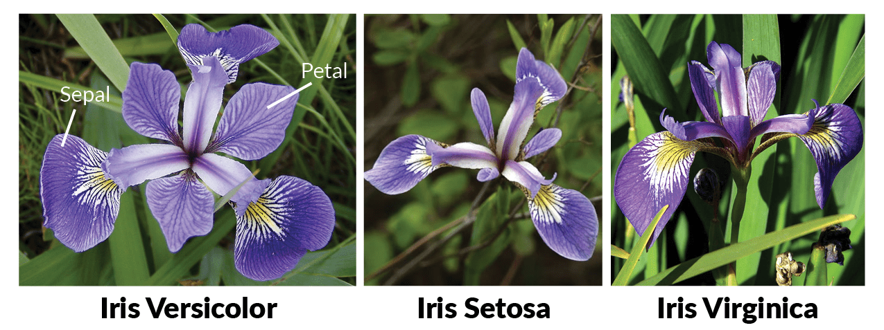

Introduced by the British statistician and biologist Ronald Fisher, the dataset consists of 50 samples for each of the three Iris flower species.

Each sample contains the length and width of sepals and petals in centimeters, making a total of four attributes. Based on the combination of these four characteristics, Fisher developed a model to distinguish one species from another.

The Iris dataset is widely used and is included in the Scikit-learn library, making it easily accessible for importing without the need to search for a download source.

Scikit-learn

Scikit-learn is a practical machine learning library organized into modules, each tailored for specific purposes.

Among the main modules, we have classification, regression, clustering, and dimensionality reduction. In the next section, we will explore how to use this library to classify Iris flower samples.

Hands-on

With the main concepts of the algorithms and tools covered, it’s time to jump into Colab and get our hands dirty

Training

Let’s start by importing the Iris dataset using the scikit-learn library (already available in Colab).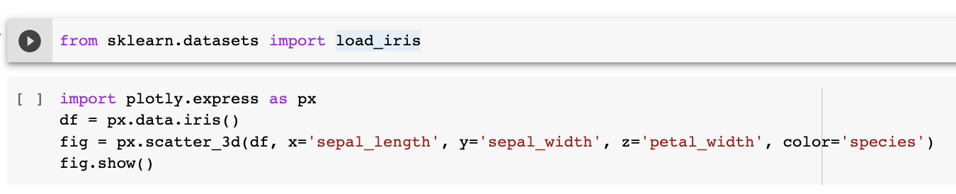

Additionally, we import Plotly Express (px) from the Plotly package, which allows us to visualize the Iris dataset in a 3D graph.

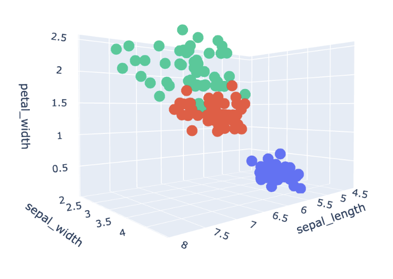
The graph displays the setosa species (in blue), the versicolor species (in red), and the virginica species (in green).

The data distribution reveals that different flower species can be distinguished by a straight line. Furthermore, we can observe that setosa flowers (in blue) have characteristics that are more distinct from those of versicolor and virginica species.

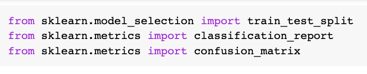
Scikit-learn already provides the KNN and K-means methods, so let’s import them!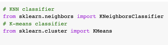

After using these methods to classify the data, we need to assess the performance of the classifiers. For this purpose, scikit-learn offers a package of evaluation metrics.

Now, we have the data and all the methods needed for classification and analyzing the algorithm results. One essential practice in machine learning is to split the dataset into training and testing data. Conventionally, the characteristics of an element in the dataset are named X, and the corresponding label or name is named y.

Thus, when dividing the data using the train_test_split function from the scikit-learn library, the sepal and petal lengths and widths of Iris flowers will be divided between X_train and X_test, while the flower names will be divided between y_train and y_test.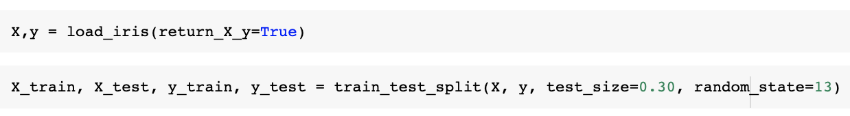

Next, we will perform flower classification using KNN. We first determine the number of neighbors (n_neighbors) and then instantiate the model that will be trained, identified by the variable “model” in the script below.

The fit function is responsible for training the model, taking the characteristics and flower names we previously divided as input parameters.

After training, we can use the model to make predictions on unknown data. At this stage, we will use the test data we separated earlier, along with the predict function.

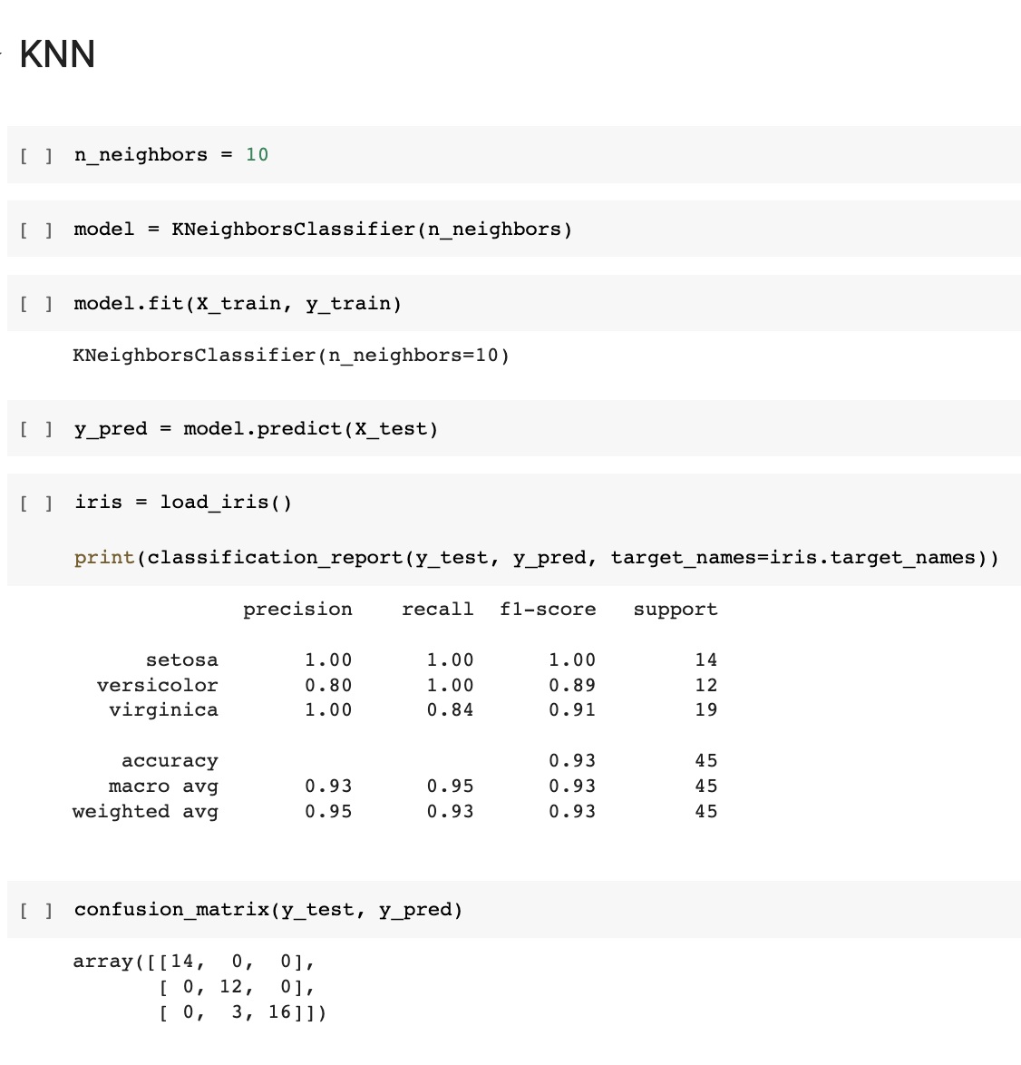
The predict function will ask the model to classify the data and return the name of each flower in the test sample.

To evaluate the model’s performance, we need to calculate several metrics, such as precision, recall, and F1-score. Scikit-learn can assist us with this through the classification_report function.

In just a few steps, we were able to train a model using the KNN method with the support of the implementations available in the scikit-learn library.

Another advantage of using this library is its standardization, which allows for easy adaptation when using other methods.

In the following script, let’s see how to classify the Iris flowers using K-means.

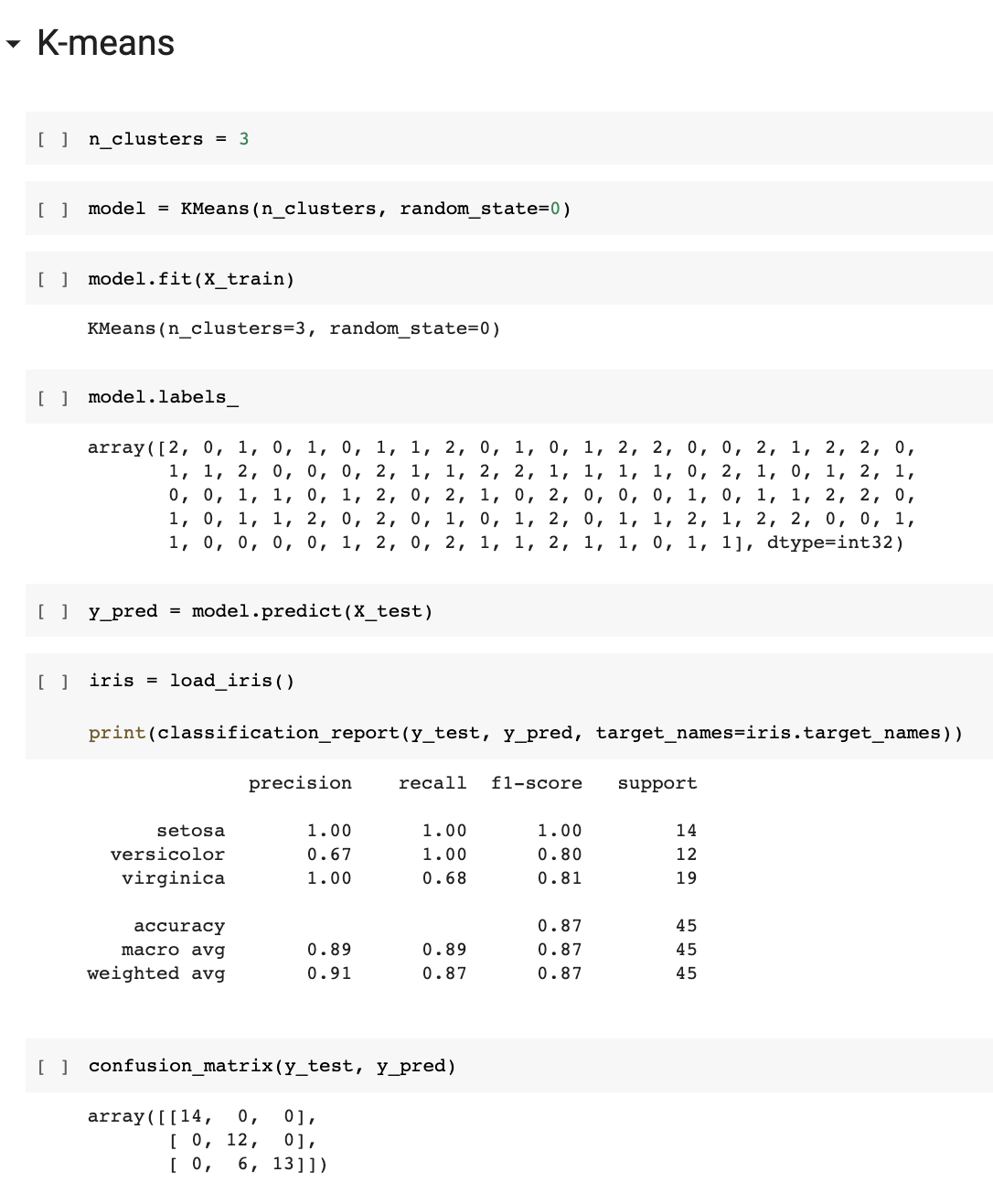
The only difference in terms of code between the two methods is the model instantiation. As the parameters and functioning of each algorithm are different, this reflects in the model creation. However, other steps, such as training and metric evaluation, remain standardized by the scikit-learn library.

This standardization contributes to the process of discovering which method provides the best performance for the problem we aim to solve, making it relatively easy to train a series of distinct methods.

Evaluation metrics

It’s essential to evaluate the model’s performance after training, isn’t it?

Let’s briefly understand the meaning of each metric calculated in the previous step. Here we go!

The performance of machine learning methods can be measured through True Positives (TP), True Negatives (TN), False Positives (FP), and False Negatives (FN) values.

These values form what we call the Confusion Matrix, represented by the confusion_matrix function in our script. ;p

The Confusion Matrix serves as the foundation to calculate the metrics used in this example: precision (true positive rate), recall (true positive rate within the positive class), and F1-score (weighted harmonic mean between precision and recall).

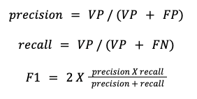
These metrics are well-established measures in the literature. So, we don’t need to worry much about their origins, but we should understand what each one represents regarding our model’s performance.

How about discussing evaluation metrics further in a future post? Sounds like a plan!

Conclusions

In this article, we explored how to use the KNN and K-means methods with the support of the scikit-learn library. We also discovered some useful functions available in the library, such as calculating performance metrics for the trained model.

Through the calculated metric report, we observed that both methods were highly effective in classifying the Iris flower species. The KNN method achieved F-scores of 100%, 89%, and 91% for the setosa, versicolor, and virginica species, respectively. Meanwhile, the K-means method achieved values of 100%, 80%, and 81%.

It’s crucial to consider which metric is most relevant for each problem, as well as the impact of the parameters used in each method’s instantiation on its performance. Therefore, defining an experiment protocol to achieve the best result for each evaluated method is essential.

References:

Müller, Andreas C., and Sarah Guido. Introduction to machine learning with Python: a guide for data scientists. O’Reilly Media, Inc., 2016.

R. A. Fisher (1936). The use of multiple measurements in taxonomic problems. Annals of Eugenics. 7: 179-188.

UCI Machine Learning Repository: Iris Data Set.

Machine Learning in R for beginners